Getting Started

MassFlow is a modular computing framework for mass spectrometry imaging (MSI) and mass spectrometry (MS) data. It provides efficient data loading, preprocessing, and data-management functions.

Authors: Leqiang Dong, Jingwei Dong

Feedback: If you find any problems while using MassFlow or reading the documentation, you can submit feedback through GitHub Issues, or contact us by email at 707244007@qq.com.

Overview

MSI datasets usually contain large numbers of pixels and mass-spectrometry measurements. Direct analysis can be affected by background signals, noise, peak-position shifts, and low-quality peaks.

MassFlow integrates commonly used MSI preprocessing steps into a single workflow. Users only need to provide the data files and select the processing steps they want to run to generate a new MSI dataset.

It is suitable for:

• MSI, metabolomics, and mass-spectrometry researchers who want to preprocess imZML data;
• users who want to perform peak picking, peak alignment, isotope filtering, adduct filtering, or statistical filtering;
• users who want to further inspect ion images or perform UMAP/KMeans-based tissue-region analysis.

What MassFlow Can Do

• Read MSI data — Directly read .imzML and .ibd files for subsequent processing.
• Baseline correction — Remove background signals that change slowly with m/z.
• Noise reduction — Reduce random fluctuations in spectra so that true peaks become clearer.
• Intensity normalization — Reduce differences in overall signal intensity between pixels.
• Peak picking — Identify major ion peaks from profile spectra.
• Peak alignment — Map nearby peaks from different pixels to common m/z positions.
• Peak filtering — Remove selected duplicate or low-quality peaks based on isotope relationships, adduct relationships, or statistical characteristics.
• Spatial analysis — View ion images and use UMAP/KMeans to help inspect different tissue regions.

1. Install MassFlow

MassFlow requires Python 3.12 or later. Before installation, first check your Python version.

Open PowerShell and run:

python --version

The current Python version will be displayed, for example:

Python 3.12.13

If the displayed version is lower than Python 3.12, install or switch to Python 3.12 or later first.

If Python 3.12 or later is displayed, you can continue with the installation.

After confirming the Python version, run the following command in the terminal:

pip install massflow

MassFlow will be installed into the environment associated with the current Python installation.

After installation, run:

python -c "import massflow; print('MassFlow installed successfully')"

Check whether MassFlow has been installed successfully.

If you see:

MassFlow installed successfully

MassFlow can now be imported normally.

2. Read imZML Data

MassFlow can read imZML data commonly used in mass spectrometry imaging.

An imZML dataset usually consists of two files with the same file name:

example.imzML
example.ibd

where:

• the .imzML file mainly stores data descriptions and the spatial position corresponding to each mass spectrum;
• the .ibd file stores the actual m/z and intensity data.

In mass spectrometry imaging data, it can be simply understood that each acquisition position in the tissue corresponds to one mass spectrum, and each mass spectrum also has its own spatial coordinates.

Therefore, an imZML dataset contains not only mass spectral signals but also the spatial relationships between these spectra in the tissue.

The two files must use the same file name and be stored in the same folder, for example:

data/
├── example.imzML
└── example.ibd

When reading the data, only the path to the .imzML file needs to be specified:

from massflow.data_manager import MSDataManagerImzML

dm = MSDataManagerImzML(
    filepath="data/example.imzML"
)

dm.load_head_data()

Here:

data/example.imzML

is only an example path and should be replaced with the actual location of your file.

You do not need to specify the .ibd file separately, as long as the corresponding .ibd file has the same file name as the .imzML file and is stored in the same folder.

3. View Basic Data Information

After running:

dm.load_head_data()

MassFlow automatically displays basic information about the MSI dataset in the terminal or Jupyter output area.

The following figure shows an example of the automatically displayed MSI data information:

When using MassFlow for the first time, you do not need to understand all of the information. You can first focus on the following fields:

• meta_profile_spectrum: Indicates whether the data are profile data. It outputs True for profile data and False for centroid data.
• meta_max_count_of_pixels_x: Number of pixels in the X direction.
• meta_max_count_of_pixels_y: Number of pixels in the Y direction.
• meta_pixel_size_x: Pixel size in the X direction.
• meta_pixel_size_y: Pixel size in the Y direction.
• meta_continuous: Indicates whether different pixels use the same m/z axis. It outputs True if the pixels share the same m/z axis and False otherwise.
• meta_mask: Spatial matrix size of the MSI data.

For example:

meta_profile_spectrum: True

indicates that the data are profile data.

meta_max_count_of_pixels_x: 227
meta_max_count_of_pixels_y: 93

indicates that the pixel range of the current data is 227 × 93 in the X and Y directions.

meta_pixel_size_x: 100.0
meta_pixel_size_y: 100.0

indicates that the pixel size is 100.0 in both the X and Y directions.

meta_continuous: True

indicates that different pixels use the same m/z axis.

meta_mask: (93, 227)

indicates that the spatial matrix size of the current MSI data is 93 × 227.

3.1 profile and centroid Data

Based on the format in which mass spectrometry signals are stored, data can generally be classified into profile and centroid types.

Profile data retain the spectrum lines obtained from continuous acquisition, allowing for the observation of relatively complete peak shapes. This format is typically suitable for processing tasks such as noise suppression, baseline correction, and peak extraction.

Centroid data primarily retain the positions and corresponding intensities of identified peaks; they typically contain fewer data points and are better suited for subsequent processing such as peak alignment and peak filtering.

3.2 continuous and processed Data

imzML can also be classified as “continuous” or “processed” based on how the m/z axis is organized across different pixels.

Continuous data indicates that different pixels use the same set of m/z positions. In other words, mass spectra from different spatial locations share the same m/z axis, with only the signal intensities varying across locations.

In processed data, different spatial locations can have their own m/z positions. Therefore, when searching for a target ion in processed data, it is typically necessary to look for positions close to the target m/z in each mass spectrum separately.

3.3 Random Spectrum Information

After displaying the MSI metadata, MassFlow also randomly selects one mass spectrum for inspection, for example:

where:

• Random Index: The index of the randomly selected spectrum.
• MS len: The number of data points contained in this spectrum.
• MS range: The m/z range covered by this spectrum.
• MS coord: The spatial coordinates of this spectrum in the MSI data.
• max intensity: The maximum signal intensity in this spectrum.

For example:

MS range: 400.0 - 1000.0

indicates that this spectrum covers an m/z range of 400–1000.

MS coord: (90, 36, 1)

indicates that this spectrum corresponds to the spatial coordinates (90, 36, 1).

This is a randomly selected spectrum and is mainly used to quickly check whether the data have been read correctly. It should not be considered representative of the entire MSI dataset.

4. View a Raw Mass Spectrum

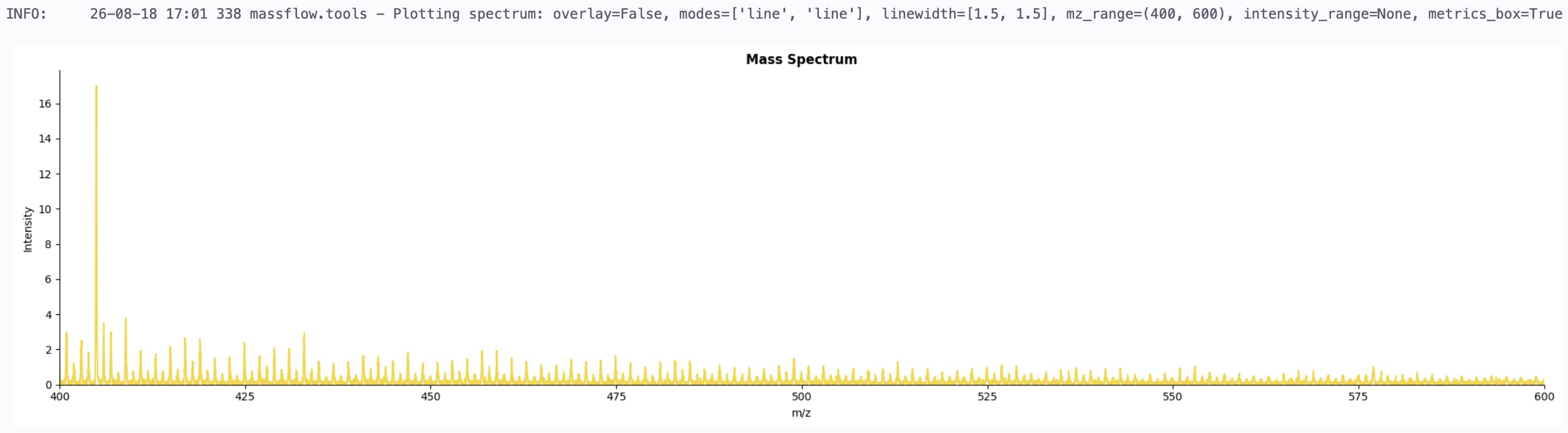
After confirming that the data have been loaded successfully, you can first plot one mass spectrum to visually inspect the raw signal.

In a mass spectrum:

• the horizontal axis represents m/z;
• the vertical axis represents signal intensity.

First import the plotting function:

from massflow.tools.plot import plot_spectrum

For example, to view the mass spectrum corresponding to one pixel:

plot_spectrum(
    dm.ms[1],
    mz_range=(400, 600),
)

Here:

dm.ms[1]

selects the mass spectrum corresponding to one pixel position.

mz_range=(400, 600)

means that only the m/z range from 400 to 600 is displayed. This range can be adjusted according to your data.

If the data are profile data, the mass spectrum is usually displayed as a continuous curve. If the data are centroid data, the plot mainly shows the positions and corresponding intensities of ion peaks.

When viewing a raw mass spectrum, you can first check:

• whether there is an obvious elevated or slowly drifting baseline;
• whether the continuous spectrum contains many rapid small fluctuations;
• the approximate m/z ranges where the major ion peaks are located.

The selected spectrum represents only one pixel and cannot represent the entire MSI dataset. In actual analysis, spectra from multiple tissue positions should be examined.

For more plotting options, including setting display ranges, plotting profile and centroid spectra, and comparing spectra before and after processing, see Spectrum Visualization.

5. View the TIC Image

In addition to examining mass spectra from individual pixels, a TIC image can be used to observe the overall spatial characteristics of the MSI dataset.

TIC (Total Ion Current) represents the sum of all signal intensities in the mass spectrum at each pixel position. By placing the TIC value of each pixel back into its original spatial position, a two-dimensional TIC image can be generated.

First import the plotting function:

from massflow.tools.plot_ion_image import plot_tic_image

Then run:

plot_tic_image(
    dm,
    output_path="tic_image.png",
    save_image=True,
    show=True,
)

The TIC image can help you inspect:

• the approximate outline of the tissue;
• blank regions;
• regions with abnormally high signals;
• obvious gaps in the scan.

The TIC image is mainly used to observe the overall spatial characteristics of the dataset and should not be used alone to determine the biological significance of a specific ion.

To examine the spatial distribution of a target m/z in the tissue, you can further generate an ion image. See Ion Image Reading and Visualization for details.

Next Steps

After reading the data and checking the basic information, raw mass spectra, and TIC image, select the subsequent processing methods according to the actual condition of the current dataset.

Common processing steps provided by MassFlow include:

Processing step	Main purpose
Baseline correction	Correct obvious baseline elevation or slow baseline drift
Noise reduction	Reduce rapid small fluctuations in profile spectra
Intensity normalization	Reduce differences in overall signal intensity between pixels
Peak picking	Identify major ion peaks from profile data
Isotope peak filtering	Reduce subsequent isotope peaks when needed
Peak alignment	Match peaks at similar positions across different pixels to a shared m/z axis
Statistical peak filtering	Further filter peaks according to their occurrence and intensity
Adduct filtering	Identify and filter different adduct ions that may originate from the same compound

When processing a new MSI dataset for the first time, it is not recommended to immediately run the entire preprocessing workflow after loading the data.

Instead, first inspect the raw data and process the data step by step in Jupyter Notebook. After each step, check the result before deciding whether to adjust the parameters or continue to the next step.

For a complete processing example, see: Best Practices